5. TESTING ASSUMPTIONS
TESTING ASSUMPTIONS
To examine the assumptions and the normality, the total scores of CIUS and OPLIS will be used. There are a few assumptions that needs to be examined which are:
a) Variable Type – the variable type used for this test is scale variable. Both the predictor and the outcome variable are qualitative and continuous in nature.
b) Non-Zero Variance – Data collected are different between each participant.
c) Independence – Each data were collected from 40 different participants showing independence of data.
d) Normality - This could be tested by using SPSS. Click 'Analyze' > 'Descriptive' > 'Explore'
The output are generated as below. Each scale will be analyzed for normality.
i) OPLIS
Based on the results shown, the graph showed a bell shaped distribution which indicated an approximately normally distributed data and the histogram showed a slight positive skewness. From the descriptive table, the skewness and the kurtosis was identified by hand calculations. The skewness is 1.235 and the kurtosis is -0.448 which shows that the assumption of normality is met. From the Shapiro-Wilk test, p = 0.067 suggesting that the data for the scale is normally distributed. The Q-Q Plot shows the dots are aligned close to the straight line and the boxplot indicated that there are no outliers. Therefore, the data can be seen as normally distributed
To examine the assumptions and the normality, the total scores of CIUS and OPLIS will be used. There are a few assumptions that needs to be examined which are:
a) Variable Type – the variable type used for this test is scale variable. Both the predictor and the outcome variable are qualitative and continuous in nature.
b) Non-Zero Variance – Data collected are different between each participant.
c) Independence – Each data were collected from 40 different participants showing independence of data.
d) Normality - This could be tested by using SPSS. Click 'Analyze' > 'Descriptive' > 'Explore'
The output are generated as below. Each scale will be analyzed for normality.
i) OPLIS
Figure: Descriptives table
Figure: Test of Normality table
Figure: Histogram
Figure: Normal Q-Q Plot
Figure: Detrended Normal Q-Q Plot
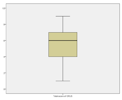
Figure: Boxplot
Report:
Based on the results shown, the graph showed a bell shaped distribution which indicated an approximately normally distributed data and the histogram showed a slight negative skewness. From the descriptive table, the skewness and the kurtosis was identified by hand calculations. The skewness is -1.447 and the kurtosis is -0.909 which shows that the assumption of normality is met. From the Shapiro-Wilk test, p = 0.013 suggesting that the data for the scale is not normally distributed. The Q-Q Plot shows the dots are aligned close to the straight line and the boxplot indicated that there are no outliers. Therefore, the data can be seen as normally distributed.
ii) CIUS
Figure: Descriptives table
Figure: Histogram
Figure: Normal Q-Q Plot
Figure: Detrended Normal Q-Q Plot
Figure: Boxplot
Based on the results shown, the graph showed a bell shaped distribution which indicated an approximately normally distributed data and the histogram showed a slight positive skewness. From the descriptive table, the skewness and the kurtosis was identified by hand calculations. The skewness is 1.235 and the kurtosis is -0.448 which shows that the assumption of normality is met. From the Shapiro-Wilk test, p = 0.067 suggesting that the data for the scale is normally distributed. The Q-Q Plot shows the dots are aligned close to the straight line and the boxplot indicated that there are no outliers. Therefore, the data can be seen as normally distributed


Comments
Post a Comment